How to Compare Two Columns in Excel: Formulas, Formatting and Online Tools
Compare two Excel columns with simple formulas, COUNTIF and XLOOKUP, conditional formatting, or a free online tool that never uploads your data — step by step.
2026/08/11
Quick answer
| Method | Where it runs | Order matters? | Best for |
|---|---|---|---|
1. =A2=B2 and EXACT formulas | Excel | Yes — row by row | Aligned columns, quick TRUE/FALSE audit |
2. COUNTIF, MATCH, XLOOKUP | Excel | No — membership test | Finding values missing from the other column |
| 3. Conditional Formatting | Excel | No (Duplicate/Unique rules) | Highlighting matches in place, no helper column |
| 4. Online comparison (no upload) | Your browser, locally | Either | Instant set operations, or comparing whole files |
Every one of these beats reading down both columns by eye — whether it's last month's customer list against this month's, a product export against the warehouse count, or a mailing list against the unsubscribe file, after a few hundred rows you'll vouch for values that were never there. Which of the four methods fits depends on one question above all: do your rows line up, or do you only care whether each value exists somewhere in the other column?
Method 1: Quick formulas for row-by-row checks
When row 2 in column A is supposed to match row 2 in column B — two exports of the same records, a before-and-after of the same list — a helper column answers it in seconds:
- Click the first empty cell next to your data, say
C2. - Type
=A2=B2and press Enter. Excel returnsTRUEif the two values match,FALSEif they don't. - For readable labels, wrap it in
IF:=IF(A2=B2,"Match","Different"). - Double-click the fill handle (the small square at the cell's bottom-right corner) to copy the formula down the whole column.
- Add a filter (Data → Filter) on the helper column to show only the
FALSEorDifferentrows.
One thing to know: the = operator ignores case, so apple and Apple count as a match. When capitalization matters — part codes, case-sensitive IDs — use EXACT instead: =IF(EXACT(A2,B2),"Match","Different").
Strengths: nothing to set up, trivially auditable, and the helper column doubles as a filterable report.
Limitations: it is strictly positional. If someone inserted or deleted a single row on one side, every row below the change compares against the wrong partner and reports Different — a wall of false alarms with one real cause. Misaligned columns need Method 2 or Method 4 instead.
Method 2: Find values missing from the other column
When order doesn't matter, the real question is membership: which values in column A never appear anywhere in column B, and vice versa? Three formula families answer it — pick whichever reads best to you.
COUNTIF — the shortest test
=COUNTIF($B$2:$B$500,A2)=0 returns TRUE when A2 appears nowhere in column B. A friendlier version: =IF(COUNTIF($B$2:$B$500,A2)=0,"Missing from B",""). The $ signs keep the search range fixed as you fill the formula down — forget them and every row searches a different, shifted range.
MATCH with ISNA
MATCH returns the position of a value in a range, or the #N/A error when it's absent — which makes =ISNA(MATCH(A2,$B$2:$B$500,0)) a clean TRUE/FALSE missing-value test. The final 0 asks for an exact match; don't omit it.
VLOOKUP or XLOOKUP with a fallback
If you want to see the matched value rather than a flag: =IFNA(VLOOKUP(A2,$B$2:$B$500,1,FALSE),"Missing"). In recent versions of Excel (Microsoft 365 and Excel 2021 onward), XLOOKUP builds the fallback in: =XLOOKUP(A2,$B$2:$B$500,$B$2:$B$500,"Missing").
Whichever you choose, remember it only looks in one direction. For the full picture, mirror the formula on the other side — a second helper column testing each B value against column A.
Strengths: order-independent, works on columns of different lengths, and the results live in the sheet where you can filter, sort, and count them.
Limitations: you need one helper column per direction, absolute references are easy to fumble, and all of these functions ignore case (see the pitfalls below).
Method 3: Conditional Formatting across both columns
For a visual answer with no formulas at all:
- Select the first column's data, then hold Ctrl (Cmd on Mac) and select the second column's data as well.
- Go to Home → Conditional Formatting → Highlight Cells Rules → Duplicate Values…
- Leave the dropdown on Duplicate and click OK. Every value that appears more than once across your selection lights up — which, across two columns, means the values the columns share. Switch the dropdown to Unique to highlight values that appear exactly once, i.e. the ones the other column is missing.
There's a catch worth knowing: Duplicate counts repeats anywhere in the selection, so a value listed twice within column A gets highlighted even if column B has never heard of it. If your columns contain internal duplicates, remove them first (Data → Remove Duplicates, on a copy of the data) or use a formula-based rule instead.
Formula-based rules
Formula rules give you the precision the built-in rule lacks. Select A2:A500, choose Conditional Formatting → New Rule → Use a formula to determine which cells to format, and enter =COUNTIF($B$2:$B$500,A2)=0 — now only genuinely missing values are highlighted, internal duplicates or not. For a row-by-row visual instead, select both columns as one block (A2:B500) and use =$A2<>$B2 to paint every mismatched row.
Strengths: the answer is visible in place, updates live as you edit, and needs no helper columns.
Limitations: highlights are hard to extract — filtering by color is clumsy compared with filtering a helper column — and the built-in Duplicate rule's behavior with internal duplicates surprises almost everyone once.
Method 4: Compare online — no formulas, no upload
Sometimes you don't want to engineer a solution inside the workbook; you want the answer.
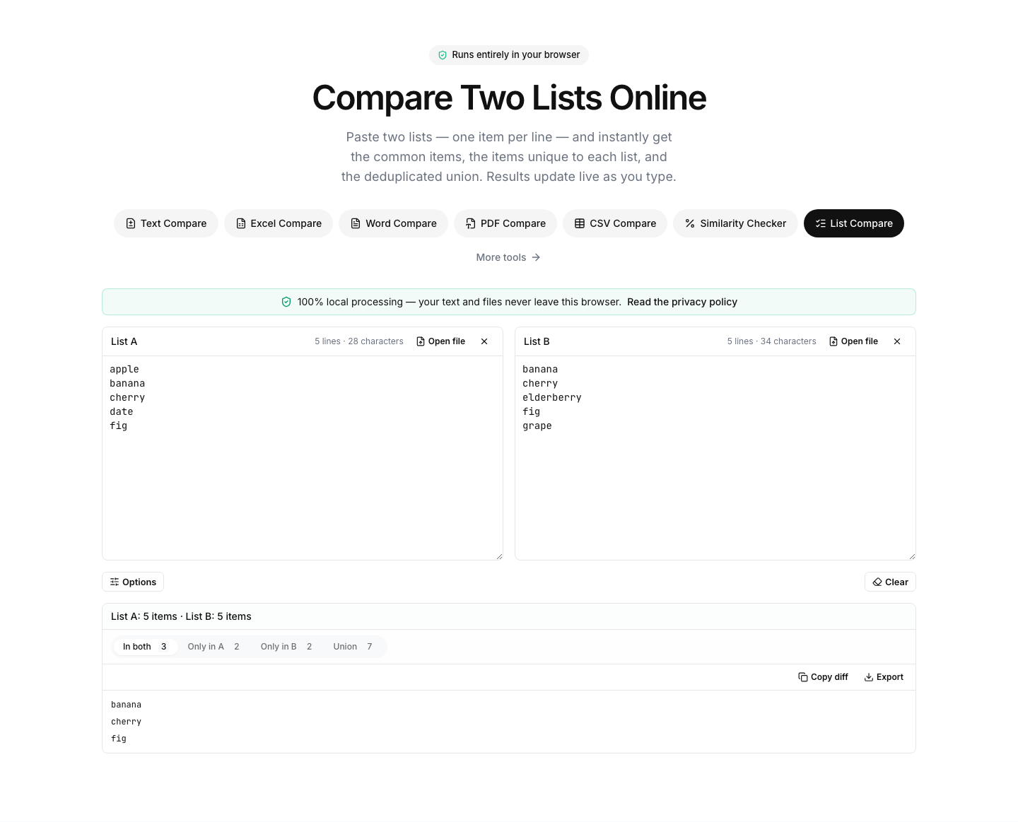
If order doesn't matter, paste both columns into the List Compare tool. Copying a column in Excel and pasting it into the browser produces one item per line — exactly what a list tool expects. The results update in real time as you paste: the values present in both columns (the intersection), the values only in the left or only in the right, and a merged, de-duplicated union you can copy back out. No $ signs, no mirrored helper columns, no rule dialogs — and duplicates are handled for you.
For row-by-row comparison — or when the columns live in two different files — use the Excel Compare tool instead. Drag in two workbooks (.xlsx, .xls, .ods, or .csv); if a workbook has several sheets, a sheet selector lets you pick the right one on each side. The rows are then compared like text, side by side with differences highlighted, and because it's a proper diff it resynchronizes after an inserted or deleted row instead of flagging everything below it — the exact failure mode of Method 1. You can ignore case or whitespace, switch between line, word, and character granularity, and export the highlighted result if you need to share it.
A note on privacy, since column comparisons are so often customer lists, payroll extracts, or account numbers: both tools run entirely in your browser. Pasted lists and opened workbooks never leave your machine, there's no account to create, and workbook parsing runs in a background worker with a progress bar, so even large files keep the page responsive.
Row-by-row check or set comparison?
This is the decision that picks your method, so make it explicitly:
- The rows are supposed to line up — same records in the same order, and you're checking a field for changes: use Method 1's formulas or the
=$A2<>$B2formatting rule; for two files, the Excel Compare tool. - Order is irrelevant — you're really asking "which values are in one list but not the other?": use
COUNTIForXLOOKUP(Method 2), Duplicate/Unique formatting (Method 3), or paste both columns into List Compare for the fastest zero-setup answer.
Choosing a positional method for a set question — or the reverse — is the root cause of most "Excel says everything is different" moments.
Frequently hit problems
Everything matches on screen but the formulas say FALSE. Almost always invisible whitespace — trailing spaces from a database export or copied web content. Compare cleaned values instead: =TRIM(A2)=TRIM(B2). Note that TRIM only removes normal spaces; text copied from web pages often contains the non-breaking space, which needs =TRIM(SUBSTITUTE(A2,CHAR(160)," ")). Online, the Excel Compare tool has an ignore-whitespace option for exactly this, and List Compare trims each item before matching by default.
Numbers that look identical won't match. If one column holds real numbers and the other holds numbers stored as text (often flagged by a small green indicator in the cell's corner), =A2=B2 returns FALSE and lookups return #N/A, because Excel treats the number 123 and the text "123" as different things. Select the text-formatted cells and use the indicator's Convert to Number option, or wrap one side in VALUE: =VALUE(A2)=B2.
Case differences slip through. =, VLOOKUP, MATCH, and COUNTIF all ignore case. If ABC-101 and abc-101 must count as different, EXACT is the go-to case-sensitive comparison in the standard formula toolkit. The Excel Compare tool is case-sensitive by default and has an ignore-case option when you want the opposite behavior.
One inserted row broke everything. A single added or deleted row makes every positional comparison below it fail. Don't fight it with formulas — switch to a membership test (Method 2) or to a diff-based comparison, which detects added and removed rows and realigns the rest.
The bottom line
For aligned columns, a helper column with =IF(A2=B2,"Match","Different") — or EXACT when case matters — is fast and auditable. For "what's missing from the other column", reach for COUNTIF or XLOOKUP with a fallback, or make it visual with Conditional Formatting's Duplicate and Unique rules. And when you'd rather have the answer than the formula: paste both columns into the List Compare tool for instant intersection, differences, and a de-duplicated union, or load two whole workbooks into the Excel Compare tool for a highlighted row-by-row diff — both free, and neither ever uploads your data.